Univariate analysis of continuous and categorical variables
2024-05-07
Source:vignettes/v01_univariate.Rmd
v01_univariate.RmdThe first step in data exploration usually consists of univariate, descriptive analysis of all variables of interest. Tidycomm offers four basic functions to quickly output relevant statistics:
-
describe()for continuous variables -
tab_percentiles()for continuous variables -
describe_cat()for categorical variables -
tab_frequencies()for categorical variables
For demonstration purposes, we will use sample data from the Worlds of Journalism 2012-16 study included in tidycomm.
WoJ
#> # A tibble: 1,200 × 15
#>    country   reach employment temp_contract autonomy_selection autonomy_emphasis
#>    <fct>     <fct> <chr>      <fct>                      <dbl>             <dbl>
#>  1 Germany   Nati… Full-time  Permanent                      5                 4
#>  2 Germany   Nati… Full-time  Permanent                      3                 4
#>  3 Switzerl… Regi… Full-time  Permanent                      4                 4
#>  4 Switzerl… Local Part-time  Permanent                      4                 5
#>  5 Austria   Nati… Part-time  Permanent                      4                 4
#>  6 Switzerl… Local Freelancer NA                             4                 4
#>  7 Germany   Local Full-time  Permanent                      4                 4
#>  8 Denmark   Nati… Full-time  Permanent                      3                 3
#>  9 Switzerl… Local Full-time  Permanent                      5                 5
#> 10 Denmark   Nati… Full-time  Permanent                      2                 4
#> # ℹ 1,190 more rows
#> # ℹ 9 more variables: ethics_1 <dbl>, ethics_2 <dbl>, ethics_3 <dbl>,
#> #   ethics_4 <dbl>, work_experience <dbl>, trust_parliament <dbl>,
#> #   trust_government <dbl>, trust_parties <dbl>, trust_politicians <dbl>
Describe continuous variables
describe() outputs several measures of central tendency
and variability for all variables named in the function call:
WoJ %>%
  describe(autonomy_selection, autonomy_emphasis, work_experience)
#> # A tibble: 3 × 15
#>   Variable            N Missing     M     SD   Min   Q25   Mdn   Q75   Max Range
#> * <chr>           <int>   <int> <dbl>  <dbl> <dbl> <dbl> <dbl> <dbl> <dbl> <dbl>
#> 1 autonomy_selec…  1197       3  3.88  0.803     1     4     4     4     5     4
#> 2 autonomy_empha…  1195       5  4.08  0.793     1     4     4     5     5     4
#> 3 work_experience  1187      13 17.8  10.9       1     8    17    25    53    52
#> # ℹ 4 more variables: CI_95_LL <dbl>, CI_95_UL <dbl>, Skewness <dbl>,
#> #   Kurtosis <dbl>
If no variables are passed to describe(), all numeric
variables in the data are described:
WoJ %>%
  describe()
#> # A tibble: 11 × 15
#>    Variable           N Missing     M     SD   Min   Q25   Mdn   Q75   Max Range
#>  * <chr>          <int>   <int> <dbl>  <dbl> <dbl> <dbl> <dbl> <dbl> <dbl> <dbl>
#>  1 autonomy_sele…  1197       3  3.88  0.803     1  4        4     4     5     4
#>  2 autonomy_emph…  1195       5  4.08  0.793     1  4        4     5     5     4
#>  3 ethics_1        1200       0  1.63  0.892     1  1        1     2     5     4
#>  4 ethics_2        1200       0  3.21  1.26      1  2        4     4     5     4
#>  5 ethics_3        1200       0  2.39  1.13      1  2        2     3     5     4
#>  6 ethics_4        1200       0  2.58  1.25      1  1.75     2     4     5     4
#>  7 work_experien…  1187      13 17.8  10.9       1  8       17    25    53    52
#>  8 trust_parliam…  1200       0  3.05  0.811     1  3        3     4     5     4
#>  9 trust_governm…  1200       0  2.82  0.854     1  2        3     3     5     4
#> 10 trust_parties   1200       0  2.42  0.736     1  2        2     3     4     3
#> 11 trust_politic…  1200       0  2.52  0.712     1  2        3     3     4     3
#> # ℹ 4 more variables: CI_95_LL <dbl>, CI_95_UL <dbl>, Skewness <dbl>,
#> #   Kurtosis <dbl>
Data can be grouped before describing:
WoJ %>%
dplyr::group_by(country) %>%
describe(autonomy_emphasis, autonomy_selection)
#> # A tibble: 10 × 16
#> # Groups: country [5]
#> country Variable N Missing M SD Min Q25 Mdn Q75 Max
#> * <fct> <chr> <int> <int> <dbl> <dbl> <dbl> <dbl> <dbl> <dbl> <dbl>
#> 1 Austria autonomy… 205 2 4.19 0.614 2 4 4 5 5
#> 2 Denmark autonomy… 375 1 3.90 0.856 1 4 4 4 5
#> 3 Germany autonomy… 172 1 4.34 0.818 1 4 5 5 5
#> 4 Switzerland autonomy… 233 0 4.07 0.694 1 4 4 4 5
#> 5 UK autonomy… 210 1 4.08 0.838 2 4 4 5 5
#> 6 Austria autonomy… 207 0 3.92 0.637 2 4 4 4 5
#> 7 Denmark autonomy… 376 0 3.76 0.892 1 3 4 4 5
#> 8 Germany autonomy… 172 1 3.97 0.881 1 3 4 5 5
#> 9 Switzerland autonomy… 233 0 3.92 0.628 1 4 4 4 5
#> 10 UK autonomy… 209 2 3.91 0.867 1 3 4 5 5
#> # ℹ 5 more variables: Range <dbl>, CI_95_LL <dbl>, CI_95_UL <dbl>,
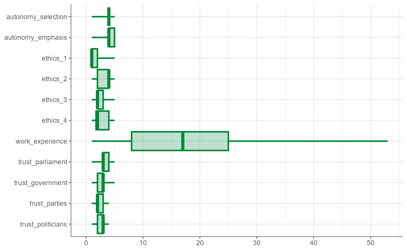
#> # Skewness <dbl>, Kurtosis <dbl>The returning results from describe() can also be
visualized:
In addition, percentiles can easily be extracted from continuous variables:
WoJ %>%
  tab_percentiles()
#> # A tibble: 11 × 11
#>    Variable            p10   p20   p30   p40   p50   p60   p70   p80   p90  p100
#>  * <chr>             <dbl> <dbl> <dbl> <dbl> <dbl> <dbl> <dbl> <dbl> <dbl> <dbl>
#>  1 autonomy_selecti…     3     3     4     4     4     4     4     4     5     5
#>  2 autonomy_emphasis     3     4     4     4     4     4     4     5     5     5
#>  3 ethics_1              1     1     1     1     1     2     2     2     3     5
#>  4 ethics_2              1     2     2     3     4     4     4     4     5     5
#>  5 ethics_3              1     1     2     2     2     2     3     4     4     5
#>  6 ethics_4              1     1     2     2     2     3     3     4     4     5
#>  7 work_experience       4     7    10    14    17    20    25    28    33    53
#>  8 trust_parliament      2     2     3     3     3     3     3     4     4     5
#>  9 trust_government      2     2     2     3     3     3     3     4     4     5
#> 10 trust_parties         1     2     2     2     2     3     3     3     3     4
#> 11 trust_politicians     2     2     2     2     3     3     3     3     3     4
Percentiles can also be visualized:
WoJ %>%
  tab_percentiles(trust_parties) %>%
  visualize()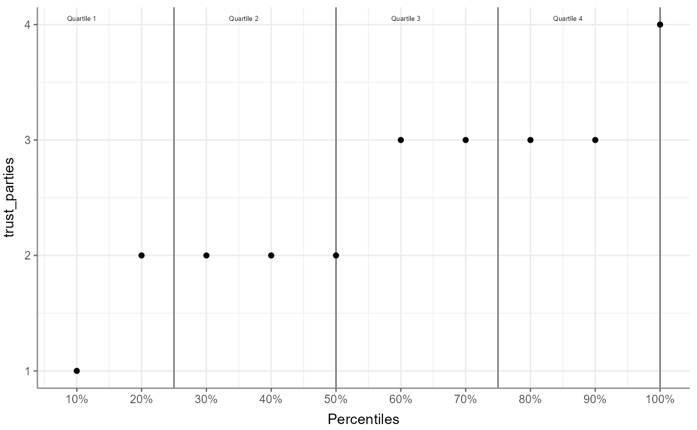
Describe categorical variables
describe_cat() outputs a short summary of categorical
variables (number of unique values, mode, N of mode) of all variables
named in the function call:
WoJ %>%
  describe_cat(reach, employment, temp_contract)
#> # A tibble: 3 × 6
#>   Variable          N Missing Unique Mode      Mode_N
#> * <chr>         <int>   <int>  <dbl> <chr>      <int>
#> 1 reach          1200       0      4 National     617
#> 2 employment     1200       0      3 Full-time    902
#> 3 temp_contract  1001     199      2 Permanent    948
If no variables are passed to describe_cat(), all
categorical variables (i.e., character and
factor variables) in the data are described:
WoJ %>%
  describe_cat()
#> # A tibble: 4 × 6
#>   Variable          N Missing Unique Mode      Mode_N
#> * <chr>         <int>   <int>  <dbl> <chr>      <int>
#> 1 country        1200       0      5 Denmark      376
#> 2 reach          1200       0      4 National     617
#> 3 employment     1200       0      3 Full-time    902
#> 4 temp_contract  1001     199      2 Permanent    948
Data can be grouped before describing:
WoJ %>%
  dplyr::group_by(reach) %>%
  describe_cat(country, employment)
#> # A tibble: 8 × 7
#> # Groups:   reach [4]
#>   reach         Variable       N Missing Unique Mode        Mode_N
#> * <fct>         <chr>      <int>   <int>  <dbl> <chr>        <int>
#> 1 Local         country      149       0      5 Germany         47
#> 2 Regional      country      355       0      5 Switzerland     90
#> 3 National      country      617       0      5 Denmark        262
#> 4 Transnational country       79       0      4 UK              72
#> 5 Local         employment   149       0      3 Full-time      111
#> 6 Regional      employment   355       0      3 Full-time      287
#> 7 National      employment   617       0      3 Full-time      438
#> 8 Transnational employment    79       0      3 Full-time       66
Again, also the results from describe_cat() can be
visualized like so:
WoJ %>%
  describe_cat() %>%
  visualize()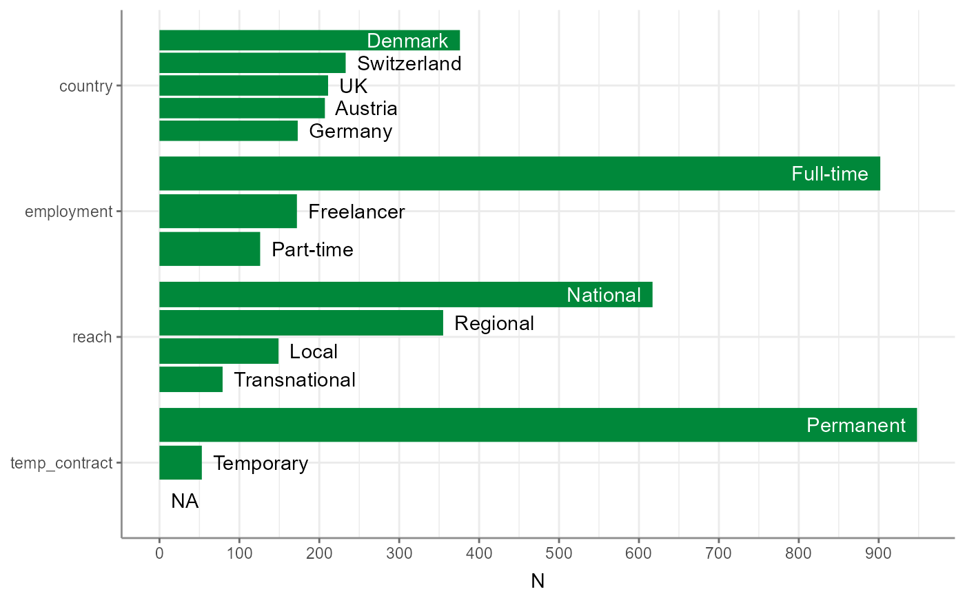
Tabulate frequencies of categorical variables
tab_frequencies() outputs absolute and relative
frequencies of all unique values of one or more categorical
variables:
WoJ %>%
  tab_frequencies(employment)
#> # A tibble: 3 × 5
#>   employment     n percent cum_n cum_percent
#> * <chr>      <int>   <dbl> <int>       <dbl>
#> 1 Freelancer   172   0.143   172       0.143
#> 2 Full-time    902   0.752  1074       0.895
#> 3 Part-time    126   0.105  1200       1
Passing more than one variable will compute relative frequencies based on all combinations of unique values:
WoJ %>%
  tab_frequencies(employment, country)
#> # A tibble: 15 × 6
#>    employment country         n percent cum_n cum_percent
#>  * <chr>      <fct>       <int>   <dbl> <int>       <dbl>
#>  1 Freelancer Austria        16 0.0133     16      0.0133
#>  2 Freelancer Denmark        85 0.0708    101      0.0842
#>  3 Freelancer Germany        29 0.0242    130      0.108
#>  4 Freelancer Switzerland    10 0.00833   140      0.117
#>  5 Freelancer UK             32 0.0267    172      0.143
#>  6 Full-time  Austria       165 0.138     337      0.281
#>  7 Full-time  Denmark       275 0.229     612      0.51
#>  8 Full-time  Germany       139 0.116     751      0.626
#>  9 Full-time  Switzerland   154 0.128     905      0.754
#> 10 Full-time  UK            169 0.141    1074      0.895
#> 11 Part-time  Austria        26 0.0217   1100      0.917
#> 12 Part-time  Denmark        16 0.0133   1116      0.93
#> 13 Part-time  Germany         5 0.00417  1121      0.934
#> 14 Part-time  Switzerland    69 0.0575   1190      0.992
#> 15 Part-time  UK             10 0.00833  1200      1
You can also group your data before. This will lead to within-group relative frequencies:
WoJ %>%
  dplyr::group_by(country) %>%
  tab_frequencies(employment)
#> # A tibble: 15 × 6
#> # Groups:   country [5]
#>    employment country         n percent cum_n cum_percent
#>  * <chr>      <fct>       <int>   <dbl> <int>       <dbl>
#>  1 Freelancer Austria        16  0.0773    16      0.0773
#>  2 Full-time  Austria       165  0.797    181      0.874
#>  3 Part-time  Austria        26  0.126    207      1
#>  4 Freelancer Denmark        85  0.226     85      0.226
#>  5 Full-time  Denmark       275  0.731    360      0.957
#>  6 Part-time  Denmark        16  0.0426   376      1
#>  7 Freelancer Germany        29  0.168     29      0.168
#>  8 Full-time  Germany       139  0.803    168      0.971
#>  9 Part-time  Germany         5  0.0289   173      1
#> 10 Freelancer Switzerland    10  0.0429    10      0.0429
#> 11 Full-time  Switzerland   154  0.661    164      0.704
#> 12 Part-time  Switzerland    69  0.296    233      1
#> 13 Freelancer UK             32  0.152     32      0.152
#> 14 Full-time  UK            169  0.801    201      0.953
#> 15 Part-time  UK             10  0.0474   211      1
(Compare the columns percent, cum_n and
cum_percent with the output above.)
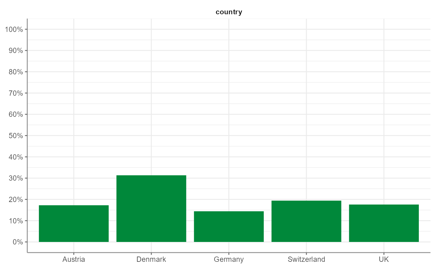
And of course, also tab_frequencies() can easily be
visualized:
WoJ %>%
  tab_frequencies(country) %>%
  visualize()